
7. Mutexes
This tutorial covers the basic use of Mutual Exclusion Semaphores (Mutex). These are particular semaphores used to 'protect' unique resources that may be used by several tasks. You'll see what this means next.
1. What's the problem?
Just try this simple application where two tasks are using the same unique hardware peripheral (USART2) to print messages over the console.
/*
 * main.c
 *
 *  Created on: 24/02/2018
 *      Author: Laurent
 */

#include "main.h"

// Static functions
static void SystemClock_Config	(void);

// FreeRTOS tasks
void vTask1 	(void *pvParameters);
void vTask2 	(void *pvParameters);

// Main program
int main()
{
	// Configure System Clock
	SystemClock_Config();

	// Initialize LED pin
	BSP_LED_Init();

	// Initialize the user Push-Button
	BSP_PB_Init();

	// Initialize Debug Console
	BSP_Console_Init();

	// Start Trace Recording
	vTraceEnable(TRC_START);

	// Create Tasks
	xTaskCreate(vTask1, "Task_1", 256, NULL, 1, NULL);
	xTaskCreate(vTask2, "Task_2", 256, NULL, 2, NULL);

	// Start the Scheduler
	vTaskStartScheduler();

	while(1)
	{
		// The program should never be here...
	}
}

/*
 *	Task_1
 */
void vTask1 (void *pvParameters)
{
	while(1)
	{
		my_printf("With great power comes great responsibility\r\n");
		vTaskDelay(20);
	}
}

/*
 *	Task_2
 */
void vTask2 (void *pvParameters)
{
	while(1)
	{
		my_printf("#");
		vTaskDelay(1);
	}
}
Again, Task_1 and Task2 are just sending messages to the console. The problem is that the message printing process in Task_1 takes 4 to 5ms. Within this delay, Task_2 is activated several times. As Task_2 has higher priority level, Task_1 is suspended while Task_2 executes.
As a result, we've got the Task_1 message cluttered with '#'... and, that's not good.

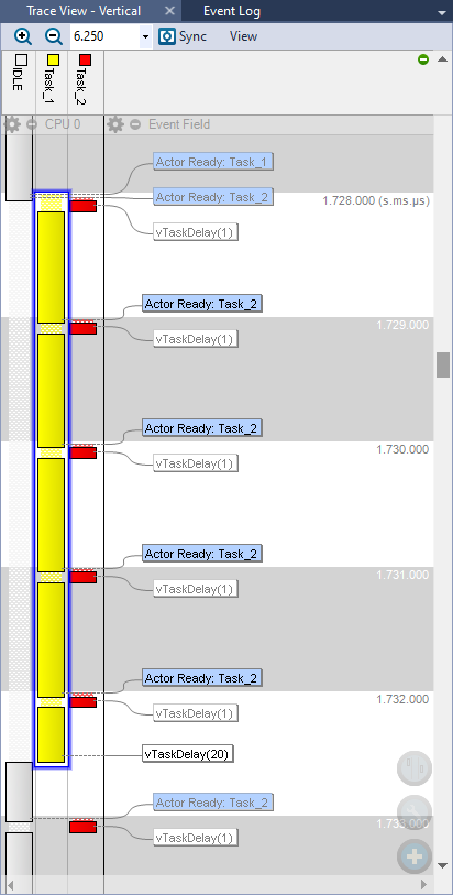
The trace record below just confirms what we already assumed. Task_1 is preempted 4 times by Task_2 after it started printing (5 if one accounts for the first preemption at the start). That corresponds well to the 4 '#' that we see in the console, in the middle of the long sentence. In theory, the number of printable characters at 115200 bauds within a 1 ms time window is:
$n=\frac{1\: ms \times 115200\: bauds}{10\: bits}\approx 11\: characters$
between the '#' which is in good agreement with what we get.
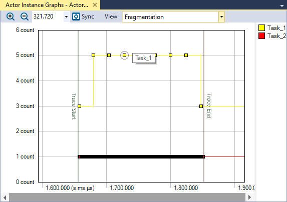
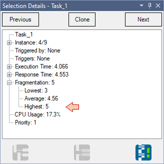
Tracealyzer offers different ways to analyze the Task_1 fragmentation. Here we see that Task_1 execution is always fragmented in 5 parts:
So can we solve this now?
Of course, inverting the priority of Task_1 and Task_2 would solve this problem. But let us assume here that this is not what we want to do. Say, Task_2 would perform some other, highly important things, and we want to keep it at a higher priority level.
2. Here comes the Mutex
2.1. Basic concepts
The problem introduced above is quite common with RTOS. It rises from a unique resource (the print peripheral here, a.k.a. USART2), either hardware (peripheral) or software (e.g. a global variables) that may be used by more than one task at a time.
There are various way to prevent such collision. An usual method is to involve a specific semaphore mechanism called Mutual Exclusion Semaphore (Mutex). Figure below illustrates the basic usage of a Mutex:
As soon as a Mutex is created, it is available. Contrary to binary semaphore, we don't have to give it first before it can be taken. You may consider a Mutex as a single token license. If you want access to a resource, you must get (take) the license first, and when you're done, you give the license back.
Task_A want to access a resource that must be protected. It tries to take the Mutex first. Since the Mutex is available the taking operation succeeds, and Task_A is now in possession of that Mutex.
Task_A is now making use of the resource. But at some point during execution, Task_B preempt Task_A, reaching for the same Mutex. Since the Mutex was taken before, the slot is empty and the take attempt from Task_B fails. Task_B then enters a blocked state waiting for the Mutex availability. Task_A resumes.
Task_A is done with the resource and give the Mutex back. At this moment, Task_B enters a ready state, waiting for the scheduler to resume its execution.
Task_B has been able to finally take the Mutex. It can now proceed with the resource.

In summary, there few usage differences between Binary Semaphores and Mutexes that are summarized below:
| Binary Semaphore | Mutexes |
|
|
2.2. Application to the protection of the console
Let us apply the above idea to our little console problem.
First, we need to make sure that Mutexes are enabled in our FreeRTOS configuration. Open FreeRTOSConfig.h and toggle the configUSE_MUTEXES to 1:
#define configUSE_PREEMPTION                    	1
#define configUSE_TICKLESS_IDLE                 	0
#define configCPU_CLOCK_HZ                      	( SystemCoreClock )
#define configTICK_RATE_HZ                      	( ( TickType_t ) 1000 )
#define configMAX_PRIORITIES                    	5
#define configMINIMAL_STACK_SIZE                	( ( uint16_t ) 128 )
#define configMAX_TASK_NAME_LEN                 	16
#define configUSE_16_BIT_TICKS                  	0
#define configIDLE_SHOULD_YIELD                 	1
#define configUSE_TASK_NOTIFICATIONS            	1
#define configTASK_NOTIFICATION_ARRAY_ENTRIES   	1
#define configUSE_MUTEXES                       	1  // <- Enable Mutexes
#define configUSE_RECURSIVE_MUTEXES             	0
#define configUSE_COUNTING_SEMAPHORES           	0
#define configQUEUE_REGISTRY_SIZE               	10
#define configUSE_QUEUE_SETS                    	0
#define configUSE_TIME_SLICING                  	0
#define configSTACK_DEPTH_TYPE                  	uint16_t
#define configMESSAGE_BUFFER_LENGTH_TYPE        	size_t
#define configHEAP_CLEAR_MEMORY_ON_FREE         	1
Then, as for binary semaphore, the first step is to declare a Mutex as global variable:
...
// Kernel Objects
xSemaphoreHandle xConsoleMutex;
...
Second, we need to create the Mutex object, within main() function:
...
	// Create a Mutex for accessing the console
	xConsoleMutex = xSemaphoreCreateMutex();

	// Give a nice name to the Mutex in the trace recorder
	vTraceSetMutexName(xConsoleMutex, "Console Mutex");
...
Note that, similar to the Binary Semaphore seen before, the xConsoleMutex variable is a pointer (4 bytes) that points to a dynamically allocated structure (*xConsoleMutex) of 80 bytes:

Finally, the Mutex can be used to 'protect' the unique resource. We basically just need to surround the use of the protected resource by the Mutex take/give operations:
/*
 *	Task_1
 */
void vTask1 (void *pvParameters)
{
	while(1)
	{
		// Take Mutex
		xSemaphoreTake(xConsoleMutex, portMAX_DELAY);

		// Send message to console
		my_printf("With great power comes great responsibility\r\n");

		// Release Mutex
		xSemaphoreGive(xConsoleMutex);

		vTaskDelay(20);
	}
}

/*
 *	Task_2
 */
void vTask2 (void *pvParameters)
{
	while(1)
	{
		// Take Mutex
		xSemaphoreTake(xConsoleMutex, portMAX_DELAY);

		// Send message to console
		my_printf("#");

		// Release Mutex
		xSemaphoreGive(xConsoleMutex);

		vTaskDelay(1);
	}
}
Once again, unlike the binary semaphore, which is usually first given and then taken by two different tasks, the Mutex is first taken, and then released (given) by the same task. It's a way for that task to say others "Hey, if you want to use the resource I'm using now, so don't interrupt me!".
Now watch the result of the above code: problem solved!

The trace below show the whole process. It is worth taking some time to understand what's happening into the details.
At t ≈ 2.112s, both Task_1 and Task_2 are ready for doing their jobs. Because Task_2 has higher priority level, it takes the Mutex, prints '#', releases the Mutex and then go to wait for 1ms. During this time, Task_1 is waiting.
Right after this, Task_1 is activated. It takes the Mutex and starts printing its long message.
At t ≈ 2.113ms, Task2 is again activated, suspending Task1. It tries to take the Mutex, but it is not available, therefore it prepares to enter the blocked state. But before doing that, something interesting happens: Since Task_1 is blocking Task_2 with the Mutex, the OS then cleverly considers that Task_1 priority level should be raised to the one of Task_2. This mechanism, called Priority Inheritance is a feature most OSTR implement. It prevents a well-known issue when using Mutexes, that arises when a third task of intermediate priority comes into the game, indirectly blocking Task_2 execution (by CPU starving Task_1) despite its lower priority level.
Right after that, Task1 resumes with its priority to the same level as the one of Task_2.
After t ≈ 2.116s, Task_1 is done printing the message and releases the Mutex. As soon as the Mutex is released, the priority of Task_1 returns to 1, and then Task_2 resumes.
Finally, both tasks enter their waiting (suspended) state.
That's beautiful, isn't it?

 | - - |